Assessing the size and uncertainty of remaining carbon budgets

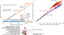
The remaining carbon budget (RCB), the net amount of CO₂ humans can still emit without exceeding a chosen global warming limit, is often used to evaluate political action against the goals of the Paris Agreement. RCB estimates for 1.5 °C are small, and minor changes in their calculation can therefore result in large relative adjustments. Here we evaluate recent RCB assessments by the IPCC and present more recent data, calculation refinements and robustness checks that increase confidence in them. We conclude that the RCB for a 50% chance of keeping warming to 1.5 °C is around 250 GtCO₂ as of January 2023, equal to around six years of current CO₂ emissions. For a 50% chance of 2 °C the RCB is around 1,200 GtCO₂. Key uncertainties affecting RCB estimates are the contribution of non-CO₂ emissions, which depends on socioeconomic projections as much as on geophysical uncertainty, and potential warming after net zero CO₂.

Similar content being viewed by others

Opportunities and challenges in using remaining carbon budgets to guide climate policy

An integrated approach to quantifying uncertainties in the remaining carbon budget

Substantial reductions in non-CO₂ greenhouse gas emissions reductions implied by IPCC estimates of the remaining carbon budget

Main

The remaining carbon budget (RCB) is the net amount of carbon dioxide (CO₂) humans can still emit while keeping global warming below a given limit with a given probability, taking into account the effect of other anthropogenic climate forcers 1,2 . The concept is key when considering the speed of decarbonization required to meet the goal of the Paris Agreement to keep global warming to well below 2 °C relative to pre-industrial levels and pursuing efforts to limit it to below 1.5 °C (ref. 3 ). Many approaches to equitable international climate action involve estimating the global RCB and dividing it among nations according to various principles of equity 4,5 . However the RCB for the Paris-relevant temperature targets (generally interpreted as a 50% chance of keeping global warming below 1.5 °C and anywhere from a 66% to 90% chance of 2.0 °C (ref. 6 )) is small compared with the uncertainty in their values. This means subtle updates to the assessments can substantially affect the values, which makes their use challenging.

Previous work shows that the temperature rise is, to first order, not strongly dependent on when carbon emissions occur, only on their cumulative sum 7,8,9,10,11,12,13 ; however, the RCB is strongly dependent on both how much and when different types of non-CO₂ emissions occur 14,15,16,17,18,19 . As a result, the RCB requires some set of scenarios describing co-evolutions of CO₂ and other emissions to estimate.

In the Working Group I (WG1) report for the IPCC Sixth Assessment Report (AR6) 1 , a set of values were established using the approach presented in refs. 19,20 , decomposing the RCB into CO₂ and non-CO₂ parts. The CO₂ part was assessed analytically by integrating information from multiple lines of evidence, while the non-CO₂ part was assessed using a reduced-complexity climate model (or emulator), MAGICC 7.5.1 21,22,23 , calibrated to the IPCC AR6 assessment 24 . The impact of non-CO₂ emissions on the RCB was estimated by fitting a linear trend to the relationship between future non-CO₂ and future total warming at net zero CO₂ emissions for available scenarios in the database accompanying the IPCC Special Report on Global Warming of 1.5 °C (SR1.5) 25 . Following an update to historical data, an updated version of MAGICC (7.5.3) was available and used in the WG3 report 26,27 .

The WG3 report discusses how updates to the non-CO₂ contribution at the time of net zero reduce the 1.5 °C RCB by about 100 GtCO₂ (about one-fifth) relative to estimates reported in WG1, although it did not tabulate values. It also makes comparisons between the RCB and the cumulative emissions until net zero of scenarios meeting a given temperature goal, which it finds approximately consistent with each other, although with less consistency for 1.5 °C of global warming than for higher levels. While this 20% change in the RCB estimate is small compared with the overall uncertainty and with past updates between the IPCC Fifth Assessment Report 8 and the SR1.5 19 , it is politically important and warrants investigation.

In this Article, we update the RCB calculations fully and include results from an additional simple climate model calibrated for use in the latest IPCC report, FaIR 24,28 . We then present improvements to the calculation methodology and examine the impact of these changes. We assess the RCBs through six contributing factors following ref. 20 and present the results of various changes in calculation that lead to updated values. Where not otherwise mentioned, RCBs are listed for keeping warming to the specified warming limits with 50% probability.

Sources of uncertainty

The main contributing factors in the budget calculation assessed by WG1 1 are transient climate response to cumulative CO₂ emissions (TCRE, the temperature rise per unit carbon emitted 2,29 ), historical warming (assessed human-induced global average temperature rise at present relative to pre-industrial levels), unrepresented Earth system feedbacks (ESFs), zero-emissions commitment (ZEC, the CO₂-based warming that continues after CO₂ emissions reach and are kept at net zero), warming from non-CO₂ emissions relative to the historical period and recent emissions. The equation combining these can be found in Methods, and a schematic of the equation is found in Fig. 1a. The values used for these variables can be found in Table 1.

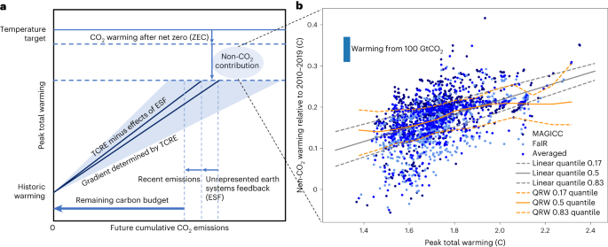
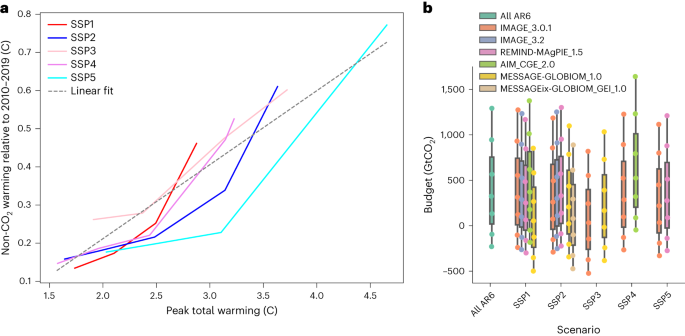
In general, scenarios are designed to limit global warming to below a certain limit. Such scenarios aim to limit all GHG emissions, often modelled by applying a CO₂-equivalent price to all GHGs. Intuitively, one therefore expects a monotonic relationship between total warming and warming from non-CO₂ GHGs. However, clear limits to reducing non-CO₂ GHGs to zero have been identified, as insufficient mitigation measures have been identified to fully eliminate them for some activities such as agriculture 43 . Aerosol forcing, which cools Earth and generally reduces as CO₂ emissions do, also reduces the strength of the expected correlation. Typically, this floor of non-CO₂ warming is already achieved in pathways that limit warming below 2.0 °C and is not markedly reduced further when aiming to limit warming further to lower levels 42 . This minimum floor of non-CO₂ emissions determines to a large degree the non-CO₂ warming expected around the time CO₂ emissions reach net zero. Importantly, this minimum floor level can differ substantially both between models and between model configurations, for example, depending on assumptions about future socioeconomic development, what mitigation options are possible in a model or how land systems are treated. While the 17–83% uncertainty range in the fit to scenario data corresponds to a change in budgets of only around 100 GtCO₂, many individual scenarios lie several times this outside this range, as seen in Fig. 1b.

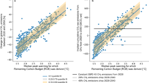
We also investigate the impact of model and SSP scenario family on RCBs (Fig. 2b). Similar plots for the SR1.5 database can be found in Supplementary Fig. 2. While results are clearly different for each combination, no clear trends emerge, assuaging concerns that overrepresentation of a few models or scenario families in the AR6 database might systematically bias the RCB calculations. This concern is also assuaged by the small impact of changing between the AR6 and SR1.5 databases (2 with scenarios from the AR6 database. The range of values across all model–SSP combinations is from 490 GtCO₂ to a minimum value of 80 GtCO₂. Carrying out the same analysis with the scenarios available in the SR1.5 database results in similar values. This emphasizes that, depending on how successfully non-CO₂ emissions are reduced, the 1.5 °C RCB can change by a factor of around two and that a more precise RCB estimate needs to be conditional on the non-CO₂ pathway to net zero. Equally, the use of RCBs to assess the global warming performance of pathways can be made more accurate if these sorts of conditional RCBs are used for comparison instead of generic central estimates.

Timing of non-CO₂ warming

The RCB is properly defined as the cumulative CO₂ emissions until annual net CO₂ emissions become zero. However, in virtually all pathways, CO₂ is the only major GHG to reach net zero. Residual emissions of other long-lived GHGs mean that Earth may continue to warm after reaching net zero. In practice, most scenarios that reach net zero CO₂ in our scenario databases then achieve net negative CO₂ emissions, and these negative emissions soon cancel out the warming from other forcers. Furthermore, both emulators used in this study have slightly negative ZECs (despite being calibrated to the IPCC AR6 assessment, which reports that the assessed value of ZEC is close to zero but with low confidence in the sign 32,33,35 ). This negative ZEC in the emulators usually prevents rises in median temperature in net zero scenarios to the end of the century. These facts defang but do not resolve the question of when we should measure the non-CO₂ warming.

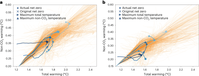
Our default definition of non-CO₂ warming is the non-CO₂ contribution to warming at the time CO₂ emissions become net zero, consistent with recent IPCC RCB estimates 1 . It has the benefit of decoupling the time used for determining non-CO₂ warming from the temporal evolution of the emulator’s temperature response. This, for example, reduces the impact of the emulator’s negative ZEC. It is, however, not the right choice of timing to ensure a given temperature is not exceeded because it does not estimate the non-CO₂ contribution at the time of peak temperature. We therefore consider variations on this assumption, described in detail in Methods and plotted for a few scenarios in Fig. 3. We find that while in some scenarios different approaches will get very similar results, in other scenarios results may differ by more than 0.1 °C. Some alternative approaches that can be considered are the non-CO₂ warming at the time of the model-reported net zero date (the date of net zero before emissions were harmonized to be consistent with recent emissions 44 ), the maximum possible non-CO₂ warming at any point over the twenty-first century and the non-CO₂ warming at maximum total temperature. The impact of changing between these measures is investigated in Table 2. Most pathways do not reach net zero and therefore do not contribute to the calculation in the first two approaches. It will generally improve results to also exclude them from other approaches since these scenarios do not reach their peak temperature during the twenty-first century and so do not have well-defined RCBs.

The maximum non-CO₂ warming is an upper bound on the non-CO₂ term (which is negative in the equation for the RCB) rather than a fair estimate. The original (before harmonization to recent observations) net zero test functions as a robustness check against any distorting impact of harmonization on pathways. Table 2 shows that the influence of this standard operation is minor. The most appropriate estimate of non-CO₂ warming comes from the estimates of non-CO₂ emissions at the time of peak warming since this is the deciding point for whether the scenario exceeds a particular limit. To combine the evidence that comes from the non-CO₂ warming estimates of MAGICC and FaIR, the temperature trends of the two emulators should be averaged before a maximum is found because otherwise the estimates may come from different years. Furthermore, viewing the two estimates as the true value plus an error term, averaging first and then finding the maximum allows more opportunities for error cancellation. We therefore consider average-first non-CO₂ warming at peak total temperature the best estimate of the marginal effect of non-CO₂ warming on the peak temperature. It is generally higher than the average non-CO₂ warming at net zero and hence decreases the 50% 1.5 °C RCB by 16% (Table 2). We use this technique in our ‘recommended update’. The temperature limit indicated by this non-CO₂ contribution is generally temporary and before peak CO₂ warming is reached; hence, the older practice (continued in our ‘default update’) of taking the contribution at net zero might be justified. The default update simply incorporates new data into the pre-existing methodology; the recommended update includes calculation methodology changes.

Comparison of recommended result with AR6 WG1 results

The RCB factors updated from the AR6 WG1 report to the approach we recommend can be summarized as follows: more recent emissions were included; the version of the climate emulator MAGICC was updated and calculations from FaIR were included; the database of scenarios was changed from SR1.5 to AR6; the non-CO₂ trend was found using QRW instead of a linear trend; and the non-CO₂ warming is taken at the time of peak total warming from scenarios that reach net zero instead of at the time of net zero. As seen in Fig. 4, recent emissions, recalibrating MAGICC and the addition of FaIR had the largest impact. The difference between recommended and previous budgets is small by 2 °C, and the updated RCB for higher degrees of warming is larger for temperature rises above 2.2 °C. A diagram of budgets with different MAGICC and FaIR versions can be found in Supplementary Fig. 1. Including a variety of emulators increases the robustness of the estimate as does making non-CO₂ assumptions explicit; applying a nonlinear relationship for estimating non-CO₂ warming as a function of total warming, choice of time for non-CO₂ warming and the database of scenarios is less impactful.

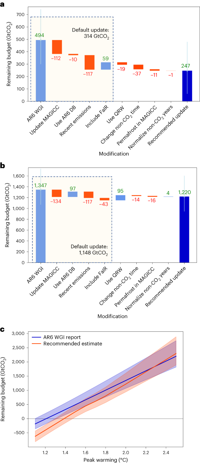
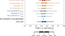
After making all these changes, our best (50%) RCB estimate starting after 2022 is 250 GtCO₂ (17–83% range from uncertainty in the impact of CO₂: −170 to 840 GtCO₂) for the RCB for limiting warming to 1.5 °C. The same uncertainty in the modelled impact of non-CO₂ forcing gives a range of 160–280 GtCO₂. We can combine these uncertainties using a generalized extreme values functional fit to the quantiles (described in Methods), resulting in a range of –200 to 830 GtCO₂. Note that the skew on non-CO₂ uncertainty lowers both limits. For 2 °C, we have 1,220 GtCO₂ (650–2,270 GtCO₂ from CO₂; 600–2,240 GtCO₂ including non-CO₂ uncertainty). For limiting warming to 2°C with 66% or 90% probability, the RCBs are estimated at 940 and 500 GtCO₂, respectively. With 40 GtCO₂ emitted in 2022 45 , this is roughly equivalent to 23 and 12 years of current CO₂ emissions for a 66% or 90% chance, respectively, of limiting warming to 2 °C and 6 years of emissions for a 50% chance of 1.5 °C. Translated into linear paths to net zero, this implies reaching global net zero CO₂ emissions around 2070, 2050 and 2035.

Methods

The equation for the RCB B for a temperature T is expressed as

For each temperature target, 10 million values for ESF, ZEC and TCRE are drawn from the relevant distributions (Table 1), assuming independence between each of the estimates, combined with the best estimate of non-CO₂ warming contribution for this level of peak warming and plugged into equation (1). Quantiles of the resulting budgets are then calculated. Where the normal distribution is used to capture the uncertainty in TCRE, it is possible to obtain a negative TCRE value. This would be an odd assumption that often results in a negative budget. However, this negative budget is the lower bound rather than the upper bound for emissions reaching that temperature target. The probability of a negative TCRE is less than 1% with our distribution based on the IPCC AR6 assessment 1 ; for this reason and for visual clarity, graphs such as Supplementary Fig. 3 do not depict the top and bottom 1% of results for any distribution. The impact of replacing these negative TCRE draws with a very small positive value (a positive-only normal distribution) is investigated in Table 2 and found to be minor for 50%–90% budgets; it is only relevant to the extreme-probability budgets. ESF is expressed as CO₂ emitted per degree of warming and is also given by a normal distribution of values multiplied by future warming; its impact is small for budgets below 2.5 °C, so we do not consider robustness checks of this. The emissions from 2020 to 2022 were not included in the WG1 budgets and were recently evaluated as amounting to 121 GtCO₂ (ref. 45 ), although changes in the estimates of emissions in earlier years mean that our recent emissions change by 131 GtCO₂.

For the non-CO₂ components of projections, we default to (and recommend using) the AR6 scenario database 38 but also investigate the use of the SR1.5 database 25 for comparison with previous IPCC RCBs. The emissions scenarios in both databases are vetted to ensure that key emissions species and socioeconomic variables are within reasonable ranges in the recent past and near future, then harmonized to match historical emissions precisely and infilled with any missing emissions 44 .

The emissions scenarios from the AR6 and SR1.5 databases are then run through reduced-complexity climate model emulators. For climate emulators, we use runs from both MAGICC 7.5.3 21 and FaIR 1.6.2 28 . By default, we use versions of the emulators calibrated to assessments in the AR6 WG1 report 24 , but we also compare these results with runs using older model versions and pre-AR6 calibrations (MAGICC 7.5.1 and FaIR 1.3.4) for robustness checks. Both versions of MAGICC also have the option of including a module designed to mimic the effects of permafrost thawing; the impact of turning this option on is also investigated. Note that this affects only the relationship between total warming and non-CO₂ emissions as the feedback of permafrost melting on the warming per unit of CO₂ is included in the ESF.

The non-CO₂ warming contribution is calculated slightly differently in FaIR and MAGICC. In FaIR, we calculate the warming from only anthropogenic emissions and the warming from the same scenarios with only anthropogenic CO₂ emissions. We subtract the average temperatures in the period 2010–2019 from each case, and the difference between these values is then the non-CO₂ contribution to warming. In MAGICC, we do three experiments for each scenario: one with all emissions and natural climate forcers, one with anthropogenic forcers only and one with anthropogenic CO₂ emissions only. The difference between the all anthropogenic forcers and anthropogenic CO₂-only experiments is the non-CO₂ contribution to warming. We use a different approach to MAGICC when processing FaIR data because by default, FaIR includes the effects of a substantial solar cycle in future temperatures, which we avoid including. Precalculated MAGICC and FaIR results for all these cases are included in the codebase for running these calculations.

In all cases, the peak temperature in the emulator until 2100 is compared with the non-CO₂ warming at various times, depending on the non-CO₂ peaking definition (see discussion in main text). The default peaking choice, in keeping with previous work, is the non-CO₂ warming at the time the scenario actually reaches net zero in the harmonized emissions, but we also consider the time it originally reached net zero CO₂ before CO₂ emissions were harmonized to recent historical data (non-CO₂ warming at original net zero CO₂); the non-CO₂ warming at peak total warming, either in all cases or restricted to scenarios that make net zero (after harmonization); the non-CO₂ warming at the time of peak total warming in MAGICC, conditional on meeting net zero (after harmonization); and, very conservatively, the maximum non-CO₂ warming experienced in the twenty-first century. While non-CO₂ warming at net zero CO₂ is defined only for emissions trajectories that reach net zero CO₂ (either before or after harmonization), it can also be calculated for scenarios that never reach net zero. These scenarios typically are either high warming, and hence less relevant for low-warming calculations, or nearly reach zero, meaning the difference between approaches is smaller.

Whichever value of non-CO₂ warming is used, the rest of the calculation is the same. If both MAGICC and FaIR are used, the peak warming and non-CO₂ warming are averaged before the fit to the relationship is made, as seen in Fig. 1b.

There are several ways of fitting a relationship of non-CO₂ warming contribution to total warming at peak. The default method is a linear trend, which fits a straight line to the points using quantile regression to find the 50th percentile. This is preferred to a least-squares fit, which would be more influenced by extreme points. Alternatively, this fit can be performed using a QRW method, which weights points according to 1/(1 + Δx 2 ) for Δx the distance along the x axis, normalized by a value proportional to the total range of x values. With this weighting, weighted quantiles are evaluated at ten points equally spaced across the x axis, and results for points in between are linearly interpolated. See ref. 46 for more details on this method. This technique is reasonably similar to calculating the rolling quantiles of points but with smoother behaviour and defined over a wider x-axis interval. A third technique is linear interpolation, which is appropriate only when few data points are available. We linearly interpolate between these known points to find the non-CO₂ warming corresponding to this total temperature rise, with total temperatures outside the known range assumed to have non-CO₂ warming equal to the closest point.

For runs where only a single model/scenario family is used, we filter the database for each specific model and then look for cases with at least three scenarios with names starting ‘SSPn’ for n between 1 and 5. We calculate the non-CO₂ component using the non-CO₂ warming at peak total warming of these cases, not filtering out scenarios that do not reach net zero to avoid a lack of data. Linear interpolation is used to make the fit.

To combine errors from CO₂ and non-CO₂ physical uncertainty, we fit a generalized extreme value distribution (GEV) to the quantiles of the data for each at each relevant temperature, following the approach of ref. 47 . For the CO₂ error (the largest contribution), we fit the GEV to the 0.1, 0.17, 0.33, 0.5, 0.66, 0.83 and 0.9 quantiles of standard runs. For the non-CO₂ uncertainty, we make runs using the 0.17, 0.5 or 0.83 non-CO₂ warming temperature quantiles for each scenario. Fits to the scenario warming are made as before and budgets calculated. A GEV fit to the 50% probability budget as a function of the non-CO₂ quantile is made, and to convert this into an uncertainty, we subtract that value at 0.5 non-CO₂ warming. The combined error is then determined by adding a million draws from the two GEVs together and calculating the relevant quantiles of the result.